The wrong batch size is all it takes

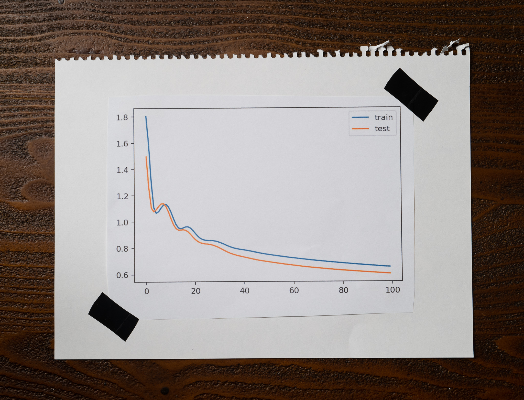
Look at this plot:

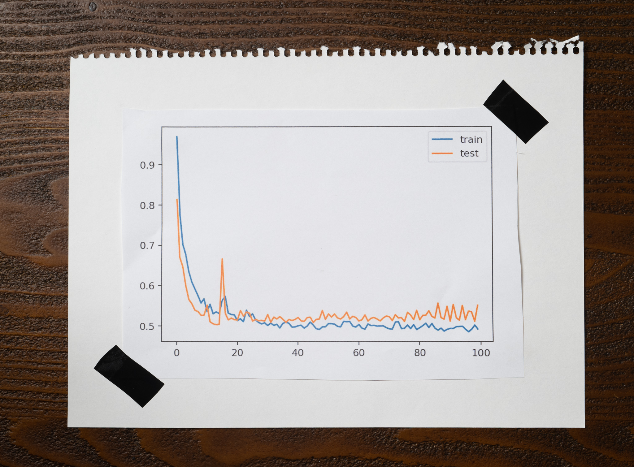
Now, compare it to this one:

They are very, very different. However, these plots come from the same place.

These are the training and testing losses of two simple neural networks that use the same architecture, trained on the exact data for 100 epochs, using the same optimizer, learning rate, momentum, and loss function.

Almost everything is the same.

Almost.

What's happening?

I'm using a different batch size.

Something that may appear as a simple difference can completely change the results of a model.

I wrote some code to try and understand how we can get such wildly different results by simply varying the batch size we use to train a model, but before, we need to think about how gradient descent works.

To train a network, we run gradient descent for multiple iterations, or "epochs." On every iteration, the algorithm computes how much we need to adjust the model to get closer to the desired results. To do this, we take samples from the training dataset, run them through the model, and determine how far away the results are from the ones we expect. We call this difference "loss" and use it during backpropagation to update the model weights.

During this process, we must decide how many training samples we'll use to compute the loss. We call this the "batch size."

We have three choices:

1. We could use a single sample to compute the loss.
2. We could use the entire training set, all the data at once.
3. We could use a few samples, more than one, but fewer than the whole training set.

Let's jump into the code to understand how different batch sizes affect our models.

The setup

The code is straightforward and starts by importing the libraries I need. I'm using a combination of Scikit-Learn and Keras to create a dataset, train, and evaluate the three models.

import matplotlib.pyplot as plt

from sklearn.datasets import make_blobs

from tensorflow import keras
from keras import layers
from keras import models
from keras import optimizers

The first step is to come up with a random dataset. I used Scikit-Learn's make_blobs() to do that:

n = 1000
classes = 3
dimensions = 2

train_size = int(n * 0.8)

X, y = make_blobs(
    n_samples=n, 
    centers=classes, 
    n_features=dimensions,
    cluster_std=2
)

X_train, X_test = X[:train_size, :], X[train_size:, :]
y_train, y_test = y[:train_size], y[train_size:]

Notice that I'm creating three classes, so this will be a multi-class classification problem. Two different features to keep it simple, and I'm generating 1,000 samples. I'll use 80% of those samples to train the model and the remaining 20% to test it.

Finally, here are two functions that I will use later on in every experiment:

def fit_model(batch_size):
    model = models.Sequential([
        layers.Dense(32, input_dim=dimensions, activation="relu"),
        layers.Dense(classes, activation="softmax")
    ])

    model.compile(
        optimizer=keras.optimizers.SGD(learning_rate=0.01, momentum=0.9), 
        loss="sparse_categorical_crossentropy", 
        metrics=["accuracy"]
    )

    history = model.fit(
        X_train, 
        y_train, 
        validation_data=(X_test, y_test), 
        epochs=100, 
        batch_size=batch_size
    )

    return model, history


def evaluate(model, history):
    _, train_accuracy = model.evaluate(X_train, y_train)
    _, test_accuracy = model.evaluate(X_test, y_test)

    print(f"Trainining accuracy: {train_accuracy:.2f}")
    print(f"Testing accuracy: {test_accuracy:.2f}")

    plt.figure(figsize=(6, 4), dpi=160)

    plt.plot(history.history["loss"], label="train")
    plt.plot(history.history["val_loss"], label="test")
    plt.legend()
    plt.show()

The fit_model() function creates a simple neural network with one hidden layer. Then it compiles the model and then fits it with the training data. Notice how I'm passing the batch size as an argument to this function.

Finally, the evaluate() function evaluates the model on the training and testing data, prints the accuracies, and plots the loss.

The first experiment

The first experiment uses a single sample as the batch size:

model, history = fit_model(batch_size=1)
evaluate(model, history)

Using only one sample of data on every iteration to compute the loss is called "Stochastic Gradient Descent."

When you start training this model, the logs will start the following way:

Epoch 1/100 800/800 [==============================]

The 800 indicates that this model will update the model's weights 800 times. That's because we have 800 training samples! Since we are using a single sample as our batch size, the model is computing the loss and updating the weights 800 times! Not surprising, this experiment is the most computationally expensive of all three.

When I ran the experiment, it took almost 200 seconds to complete. That's a long time for such a simple model with just a few data samples! Here is the plot of the training and testing losses:

Notice how much noise with the losses going up and down. Remember that the algorithm is computing the loss for every training sample, so depending on what that value is, the loss can vary dramatically, and that's what we see here.

My training accuracy for this experiment was around 0.87, while the testing accuracy was 0.85. These are low, but there's something even more interesting:

Every time I run the experiment, the accuracies look very different. Sometimes better, sometimes worse. The noise we see in the plots is probably the reason this happens.

The loss keeps jumping around, and something good about this is that your algorithm will avoid getting stuck in a local minimum when you use a tiny batch size. The swings will help it break free from suboptimal solutions! But it could have the opposite effect as well. Just like the noise helps the algorithm get away from a local minimum, it can also prevent it from settling in the global minimum.

The second experiment

The second experiment uses the entire training set to compute the loss and update the model weights:

model, history = fit_model(batch_size=train_size)
evaluate(model, history)

Using all the data at once is called "Batch Gradient Descent."

This one runs fast. Notice here how only one update happens during every epoch:

Epoch 1/100 1/1 [==============================]

When I ran it, this experiment took 4 seconds. Compare this with the 200 seconds from the previous one. It makes sense: we compute the loss and update the model's weights only once for the entire training set.

The training and testing accuracies are much better: 0.93 and 0.94, respectively. Finally, look at both losses and how smooth they are and compare them with the noisy plots from the previous experiment:

This method has a significant disadvantage: we need to store the entire training set in memory to compute the loss during every iteration. For a toy sample like this, storing all the data in memory is not a big deal, but it would be a no go for any decently sized dataset.

Finally, the lack of variability in the loss is also a problem: this method can get stuck in a local minimum, and there's nothing that will make it break free and find a better solution.

The third experiment

Let's look at the third experiment:

model, history = fit_model(batch_size=32)
evaluate(model, history)

Using some data, more than one sample but fewer than the entire training set is called "Mini-Batch Gradient Descent."

I'm using 32 samples, and that's why you see that we are doing 25 updates during every epoch: 800 divided by 32 is 25 different batches of samples:

Epoch 1/100 25/25 [==============================]

This experiment runs pretty fast as well: 10 seconds. Obviously, slower than using the entire training set but way faster than using a single sample.

The plot is beautiful:

You see some noise, but nothing compared to the first experiment. The training and testing accuracies are excellent at 0.96 and 0.94, respectively.

Mini-Batch Gradient Descent is much better at avoiding local minima, more computationally efficient than Stochastic Gradient Descent, and doesn't need as much memory as Batch Gradient Descent. But it has one disadvantage: we need to worry about an additional hyperparameter, the batch size.

The punchline

We rarely use a single sample or the entire training set in practice: both methods have significant disadvantages. Instead, we use the batch size as another hyperparameter that we can tweak to determine what's the best value for our model.

Every problem is different, but a popular recommendation is to start exploring from a relatively small batch size. For example, 32 is a good default value to get going.

By the way, interpreting learning curves is a critical skill. We can extract a lot of information by plotting and making sense of a few charts! Here is an article that uses learning curves to identify two of the most common problems in machine learning.

Here is a Google Colab notebook with the source code of the experiments from this article.